VLOOKUP to search for related information by row. For example, if you want to buy an orange, you can use VLOOKUP to search for the price.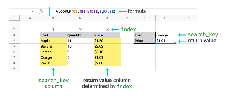
Vertical lookup. Returns the values in a data column at the position where a match was found in the search column.
Sample Usage
VLOOKUP("Apple",table_name!fruit,table_name!price)
Syntax
VLOOKUP(search_key, range,index, is_sorted)
search_key: The value to search for in the search column.search_column: The data column to consider for the search.result_column: The data column to consider for the result.is_sorted: [OPTIONAL] The manner in which to find a match for thesearch_key.FALSE: For an exact match, this is recommended.TRUE: For an approximate match, this is the default ifis_sortedis unspecified.
Tip: Before you use an approximate match, sort your search key in ascending order. Otherwise, you may likely get a wrong return value. Learn why you may encounter a wrong return value.
Tip: For more flexible database queries in BigQuery, use XLOOKUP.
Syntax
=VLOOKUP(search_key, range, index, [is_sorted])
Inputs
search_key: The value to search for in the first column of the range.range: The upper and lower values to consider for the search.index: The index of the column with the return value of the range. The index must be a positive integer.is_sorted: Optional input. Choose an option:FALSE= Exact match. This is recommended.TRUE= Approximate match. This is the default ifis_sortedis unspecified.
Important: Before you use an approximate match, sort your search key in ascending order. Otherwise, you may likely get a wrong return value. Learn why you may encounter a wrong return value.
Return value
range.| Inputs | Description |
search_key |
This is the value you search in the first column of the
range. If you expect a non-error value, the search key must be in the first column of the range. Cell reference is also supported.To do a simple check: If your
search_key is located at B3, then your range should start with column B. |
range |
This is the
range where:
To return a non-error value, your search key must be in the first column of the
range.To do a simple check: If your
search_key is located at B3, then your range should start with column B. |
index |
Also called “Column number.” This is the index of the column in the
range that contains the return value.
After you set up the range,
VLOOKUP only looks to the search key column, when index = 1 , or columns that are further right.Tip: When you use
VLOOKUP, imagine that the columns of the range are numbered from left to right and start with 1. |
is_sorted |
This is an optional input. The two available choices are
TRUE and FALSE.
We strongly recommend you:
|
| Outputs | Description |
| Return value |
This is the value that
VLOOKUP returns based on your inputs. There’s only one return value from each VLOOKUP function.
If you encounter an expected value or error like #N/A or #VALUE!, begin to troubleshoot. If you want to replace #N/A with another value, learn more about how to use IFNA() on VLOOKUP().
|
Basic VLOOKUP examples:
VLOOKUP on different search keys
Use VLOOKUP to find the price of an Orange and Apple.
When you use VLOOKUP, you can use different search keys such as "Apple" and "Orange."
range. If you don’t want to fill a value for search keys, you can also use a cell reference, for example "G9."search_key is "Orange" |
=VLOOKUP("Orange", B4:D8, 3, FALSE)
Return value = $1.01
|
search_key is "Apple" |
=VLOOKUP("Apple", B4:D8, 3, FALSE)
Return value = $1.50
|
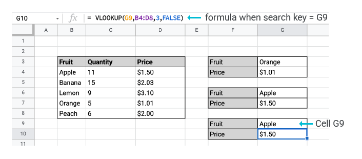
search_key that uses cell reference of "Apple" in G9 |
=VLOOKUP(G9, B4:D8, 3, FALSE)
Return value = $1.50
|
VLOOKUP on different column indexes
VLOOKUP to find the quantity of Oranges in the second index column.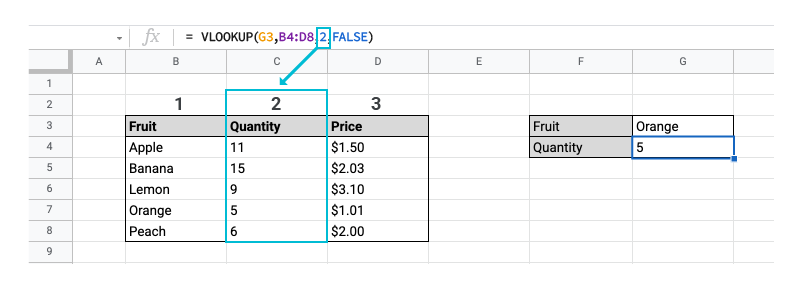
VLOOKUP, imagine that the columns of the range are numbered from left to right and start from 1. To find the target information, you must specify its column index. For example, column 2 for quantity.
Index = 2Find the quantity of oranges, which is the second column of the
range. |
=VLOOKUP(G3, B4:D8, 2, FALSE)
Return value = 5
|
VLOOKUP exact match or approximate match
- Use
VLOOKUPexact match to find an exact ID. - Use
VLOOKUPapproximate match to find the approximate ID.
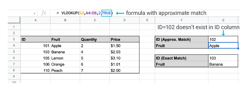
is_sorted = TRUE when you search for a best match, but not an exact match.is_sorted = FALSE, it returns an exact match. For example, the fruit name for ID = 103 is "Banana." If there’s no exact match, you get a #N/A error. Due to its more predictable behavior, we recommend you use exact match.| Exact match |
=VLOOKUP(G6, A4:D8, 2, FALSE)
Return value = "Apple"
|
| Approximate match |
=VLOOKUP(G3, A4:D8, 2, TRUE)
OR
=VLOOKUP(G3, A4:D8, 2)
Return value = "Banana"
|
Common VLOOKUP applications
Replace error value from VLOOKUP
VLOOKUP when your search key doesn’t exist. In this case, if you don’t want #N/A, you can use IFNA() functions to replace #N/A. Learn more about IFNA().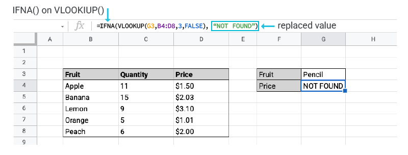
|
Originally,
VLOOKUP returns #N/A because the search key “Pencil” does not exist in the “Fruit” column.IFNA() replaces #N/A error with the second input specified in the function. In our case, it’s “NOT FOUND.” |
=IFNA(VLOOKUP(G3, B4:D8, 3, FALSE),"NOT FOUND")
Return value = “NOT FOUND”
|
Tip: If you want to replace other errors such as #REF!, learn more about IFERROR().
VLOOKUP with multiple criteria
VLOOKUP can’t be directly applied on multiple criteria. Instead, create a new helper column to directly apply VLOOKUP on multiple criteria to combine multiple existing columns.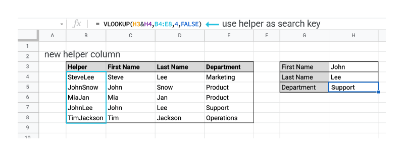
| 1. You can create a Helper column if you use "&" to combine First Name and Last Name. | =C4&D4 and drag it down from B4 to B8 gives you the Helper column. |
| 2. Use cell reference B7, JohnLee, as the search key. |
=VLOOKUP(B7, B4:E8, 4, FALSE)
Return value = "Support"
|
VLOOKUP with wildcard or partial matches
VLOOKUP, you can also use wildcards or partial matches. You can use these wildcard characters:- A question mark "?" matches any single character.
- An asterisk "*" matches any sequence of characters.
VLOOKUP, you must use an exact match: "is_sorted = FALSE".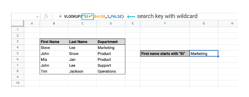
| "St*" is used to match anything that starts with "St" regardless of the number of characters, such as "Steve", "St1", "Stock", or "Steeeeeeve". |
=VLOOKUP("St*", B4:D8, 3, FALSE)
Return value = "Marketing"
|
Troubleshoot errors & best practices:
Wrong return value-
Returns an unexpected value: If you set
is_sortedasTRUE, but your first column in the range isn’t sorted numerically or alphabetically in ascending order, then change is_sorted toFALSE. - VLOOKUP gives the first match:
VLOOKUPonly returns the first match. If you have multiple matched search keys, a value is returned, but it may not be the expected value. - Unclean data: Sometimes, values with spaces that trail and lead may seem similar but
VLOOKUPtreats them differently. For example, the following are different toVLOOKUP:- " Apple"
- "Apple "
- "Apple"
VLOOKUP.- If approximate or
is_sorted=TRUEis used and if the search key inVLOOKUPis smaller than the smallest value in the first column, thenVLOOKUPreturns #N/A. - If exact match or
is_sorted=FALSEis used, then the exact match of the search key inVLOOKUPisn’t found in the first column. If you don’t want #N/A when the search key isn’t found in the first column, you can use the function IFNA().
range with a number bigger than the maximum number of columns of the range. To avoid this, make sure you:- Count the columns from the selected
range, not the entire table. - Start to count from 1 instead of 0.
- Incorrectly input the text or the column name for the
index. - Entered a number smaller than 1 for the
index. Theindexmust be at least equal to 1 and smaller than the maximum number of columns of therange.VLOOKUPcan only search in the search key column, whenindex= 1, or columns that are further right.
Important: index only accepts a number.
- You might have missed a quote in the search key when your
search_keyis text data.
| To do | Reason |
Use absolute references for range |
You should use:
You should not use:
This prevents unpredictable changes in the
range when it’s copied or dragged down. |
Sort the first column in ascending order when you use an approximate match, such as is_sorted = TRUE. |
If you use an approximate match or is_sorted = TRUE, you must sort the first column in ascending order. Otherwise, you most likely get a wrong return value. Learn more on how to sort. |
Clean your data before you use VLOOKUP |
Before you use
VLOOKUP, remember to clean your data. Unclean data may cause VLOOKUP to return an unpredictable value. Here are some common pitfalls of unclean data:
To trim white space that leads and trails, you can use Data
|
| Don't store number or date values as text |
Make sure your date or number values in the first column of your
VLOOKUP range, such as the search key column, aren’t stored as text values. You may get an unexpected return value.
|