Apr 9, 2020
How to select every nth cell in a column
Right now, when I want to open these websites, I have to hold down CTRL and then click every 5th website to select them and then when I'm done, press ALT + ENTER to open them all.
Is there a way to automate the selection part of cells?
Thanks!
Thanks!
Details
Informational notification.
This question is locked and replying has been disabled.
Community content may not be verified or up-to-date. Learn more.

Apr 9, 2020
Hi, Djordje Blagojevic,
![]()
![]()

![]()
![]()
I'll do it as below.
Test Data in B2:B.
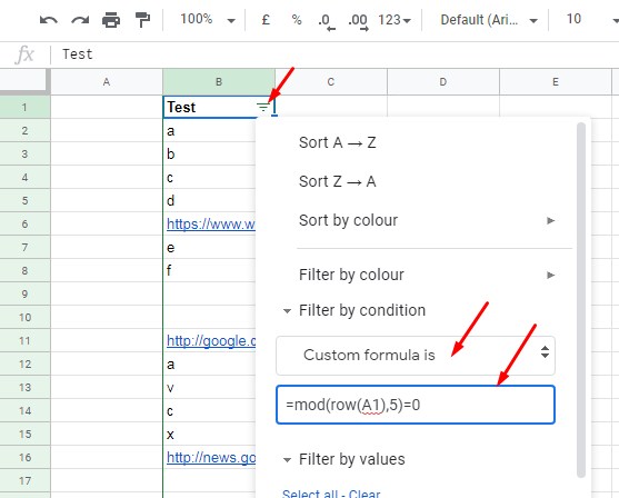
Filter Column B (select column B ->Data menu -> Create a filter).
Then use the below formula.
=mod(row(A1),5)=0
It filters every 5th row.

Select the links and hit Alt+Enter.
Hope this helps?
Best,
Prashanth KV
Last edited Apr 9, 2020
Original Poster Djordje Blagojevic marked this as an answer
Helpful?Upvote Downvote
Apr 10, 2020
You can use any cell reference like B1, C1, D1... as the below formulas will just return the same row number.
=row(A1)
=row(B1)
=row(C1)
So if the data that you want to filter is in column E, you can use the same formula, i.e. =mod(row(A1),5)=0. Change 5 to 10, to filter every 10th row.
The formula,=mod(row(A1),5)=0, works like this automatically in each row.
=mod(1,5)=0
=mod(2,5)=0
=mod(3,5)=0
=mod(4,5)=0
=mod(5,5)=0
The last formula in the fifth row would return a TRUE and the other four formulas will return FALSE.
As you may know, the MOD function returns the result of the modulo operator, the remainder after a division operation.
See the formula in the next 5 rows.
=mod(6,5)=0
=mod(7,5)=0
=mod(8,5)=0
=mod(9,5)=0
=mod(10,5)=0
Here again, only the 5th formula in row number 10 would return TRUE. So the filter filters the rows wherever TRUE appears in the test.
Refer:
Best,
Prashanth KV
Last edited Apr 10, 2020
Original Poster Djordje Blagojevic marked this as an answer
Helpful?Upvote Downvote
All Replies (4)
Hi, Djordje Blagojevic,
![]()
![]()
![]()
![]()
I'll do it as below.
Test Data in B2:B.
Filter Column B (select column B ->Data menu -> Create a filter).
Then use the below formula.
=mod(row(A1),5)=0It filters every 5th row.
Select the links and hit Alt+Enter.
Hope this helps?
Best,
Prashanth KV
Last edited Apr 9, 2020
Original Poster Djordje Blagojevic marked this as an answer
Apr 9, 2020
Could you just please explain the formula in more detail?
I don't understand why we use A1 in the formula if the data is in B column?
So if my data that I wanna filter is in column E, i have to write =mod(row(D1)5)=0, etc
You can use any cell reference like B1, C1, D1... as the below formulas will just return the same row number.
=row(A1)
=row(B1)
=row(C1)
So if the data that you want to filter is in column E, you can use the same formula, i.e. =mod(row(A1),5)=0. Change 5 to 10, to filter every 10th row.
The formula,=mod(row(A1),5)=0, works like this automatically in each row.
=mod(1,5)=0
=mod(2,5)=0
=mod(3,5)=0
=mod(4,5)=0
=mod(5,5)=0
The last formula in the fifth row would return a TRUE and the other four formulas will return FALSE.
As you may know, the MOD function returns the result of the modulo operator, the remainder after a division operation.
See the formula in the next 5 rows.
=mod(6,5)=0
=mod(7,5)=0
=mod(8,5)=0
=mod(9,5)=0
=mod(10,5)=0
Here again, only the 5th formula in row number 10 would return TRUE. So the filter filters the rows wherever TRUE appears in the test.
Refer:
Best,
Prashanth KV
Last edited Apr 10, 2020
Original Poster Djordje Blagojevic marked this as an answer