How can I keep formatting to 2 decimal spaces and / or currency when new rows are added?

The ArrayFormulas are on Row 3, starting at column V (in case that's relevant.)

ETA: Row 3 also has the correct formatting for all the columns.

(Ignore this sheet - new sample sheet bottom of thread)

you cannot format the response sheet - just pull the data to a new sheet

put your calcs & formatting there

sheet is view only

but try this on a new sheet - amend to suit your data & needs

=query('Form Responses 1'!A1:F, select A,B,E,F where A is not null order by A desc ",1)

Sorry for not replying sooner, I did not get a notification with your response.

Thank you so much for your suggestion.

I don't understand the formula (more advanced than what I normally do) - so is this supposed to keep any formatting that I choose on new rows?

Also, what is the reason the response sheet cannot be formatted? (just curious, this would help me understand.)

Thanks.

you would have to ask developer - it just defaults to bog standard arial text when new submissions come

suffise to say - response sheet is there to collect responses - just leave it to do that

as for formula

it say : simply look at (query) sheet named 'Form Responses 1'   range  A1:F

            show me columns A B E F         where A is not null (if A were text - you would say where A <>'')

            order the results by column A in descending order

I tried your query, and worked with it a few times and in a few different ways but I couldn't get it to work. Probably just more advanced than I am able to do right now.

So after trying and failing trying and failing I tried to do a simple ='Form Responses 1'!A3:A in each cell of the extra sheet that is filled out by the form.

This of course works fine if I ALREADY have a response. Then it pulls the data and I am able to do my calculations.

But it is not MAKING a new row and pulling the information into the extra sheet when a new response comes in. 

I am thinking this is precisely why you advised to do a QUERY...

Is the query the only way to have that second sheet create a new row when a response comes in?

And if so - can you give me a SIMPLER way to do the query. For example - without sorting it. It can just be an exact duplicate of how it comes in through the Google Forms.

Thanks for any additional help and guidance you may be willing to give me!

Set your sheet to editable by anyone with the link to make it easier to demonstrate solutions. Start a new new tab and enter this into cell A1, nothing anywhere else on the tab,

 

Then format the header and columns the way you want.

 

On the response tab, form responses show up in some kind of default format no matter what you do. It's just the way they have it set up. Pulling the data into another tab with this type formula allow you to format it anyway you want and it automatically brings new data over as it appears. But you must use some form of array formula, like mine, a query like Mchall's, a filter, ... a few others. Individual, row by row formulas will not bring new responses because the responses act like a new row is inserted for each response.

 

filter example

 

Personal preference as to which version you use. I like the filter but the other formula is probably the simplest if you're not comfortable with filter.

Ed

I will look through your suggestion more carefully later - thank you so much!

I just wanted to jump in here to say that I took a break, and went back to the query with fresh eyes and I got it working!

YES!

I am not sure if it's working perfectly yet, but it pulled the info. when I filled out a test response.

I don't have the calculations run yet I didn't get that far, but this is a huge step forward.

I'll be back likely tomorrow - I need to stop working on this now, I've been at it for hours.

Thank you!

It *seems* that I am pulling in the data fine, but I have another challenge.

I need/want to leave Row 3 on the Sheet 2 (Copy of Form Responses) frozen/uneditable because that's where my array formulas are (beginning AH). (Also, I'm going to be using Zapier to pull some info. from that 2nd sheet and need to make sure there are no blank rows being created at the bottom of the sheet.)

So in this case the test response - which on the Responses Sheet went into Row 4 - should have been pulled into Row 4 on Sheet 2. Then the next one would be Row 5, etc.

But that's not what happened.

 

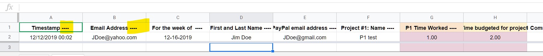
When I filled out a form, the data on Sheet 2 got pulled into Row 2 (and Row 2 seems like it's getting pulled into the headers because now all the headers have the ------- following the header names.)

I am sure part of it or most of it must be a flaw in my Query like I realize I'm pulling the header names etc., but when I tried different things like changing the range, changing the header, etc. I was still getting it wrong. 

=QUERY('Form Responses 1'!A1:AG, "", -1)

How do I change the formula so that the new data on Sheet 2 starts on Row 4, then 5, etc. (and keeping in mind i cannot have blank rows at the end of sheet)

Sample sheet  https://docs.google.com/spreadsheets/d/1P2JYVzBBUXiyDo_5PBLpEMAK7BADfOiwOCwtJ34LB5U/edit?usp=sharing 

Thanks so much for your continued help with this!

Hello CM

 Part of your problem is you erased or replaced the time stamp from A2 and A3. The query pulled the dashes into the header column because of the minus 1. Change to 1 and it will not do that.

I duplicated form response 1 and named it form response 2, then put a formula in A3 = " " so that A3 would not be blank. That's in lieu of a date in A3.

tab formatted Form Responses 2 pulls data from form responses 2 using a filter that pulls any one where column A is not blank.

tab formatted Form Responses 2A does the same thing except uses a query.

Make similar changes to form response 1 and your formula for copy of ...

Ed

I can't wait to try this! 

I had to re-read your answer several times to start to let it sink in (and will need to read again!)

I know you said in an earlier post that using a filter versus query is a matter of preference but that you prefer the filter...can you give me a couple of reasons behind your liking it better, just so I learn more how it may apply in some situations etc.

It is pulling my data in perfectly.

Thank you so much for your time and help on the sheet itself, and on the breakdown of the differences between Query and Filter, very helpful to know.

I am choosing to use Query for now only because it is what I was already using and want to move forward to the next step.

I am going to mark your suggestion as the answer.

I do have one more challenge to resolve, which I am hoping you can help with (or I can start a new thread if that's better).  For Sheet 2 - (the calculations sheet) always creates 500 rows after the new response gets pulled in which will cause an issue with Zapier.

How can I get it to not create any new rows other than the response / s?

1. In order to format the responses, the first step was to understand that the Responses needed to be kept separate from the calculations (which Mcchall C suggested)

2. To get the data pulled in correctly to Sheet 2, the formula (Query or Filter) needed to be corrected (all of the work that Ed Hannahs(Ohio) did.)

Thank you both!