Mar 9, 2021
Checkbox tick / Conditional formatting based on multiple columns
My first row is a master row that should be checked if multiple boxes in the same row of column b:d are ticked. Essentially if row 3 column b and d are ticked, column a would also be ticked, or if column c and d were ticked, column a would be ticked.
Additionally on column G I have conditional formatting where I want to make it if an episode appears on multiple disks (is checked in boxes b, c or d) then the column will turn red. I had this working when it was just 2 DVDs and cannot figure out how to make it work with 3+. Once I have 3 the rest should be easy as I just need to know if the episode appears more than once.
Sheet Link: https://docs.google.com/spreadsheets/d/1Cc4npy90_Ba8HAu7cl0kjDLK6dF0fEd5OicIfsorHC4/edit?usp=sharing
Thanks in advance for any advice.
Details
This question is locked and replying has been disabled.
Community content may not be verified or up-to-date. Learn more.
Mar 10, 2021
Hi Owen,
First, to count the unique ones (I think that means those where ONLY column D is checked), try this formula, which I've put in K2:
=QUERY(A2:D, "select count(D) where D=TRUE and B=FALSE and C=FALSE label count(D) '' ",0)It's probably pretty clear what it does, so should be easy to modify, but let me know if you have any questions.
See also the tab I added, and where I applied a data filter, just to make it easy to see only the rows with checkboxes marked. Currently, I'm showing all rows with column D checked.
Then, to explain the formula in A1:
={"M"; ArrayFormula( IF( (--B2:B)*(--C2:C) + (--B2:B)*(--D2:D) + (--C2:C)*(--D2:D) >0, TRUE,FALSE))}To be able to put the formula up in the "header" row, instead of in the first data row, which is typically done, I needed to included the header label, ie. "M"
So I start by building a virtual array, {....}, which is going to fill multiple cells, in this case the whole of column A.
So the first element in the virtual array is the header, "M", followed by a semi-colon to jump down to the next row. (To learn more about virtual array's, read this post by our expert Lance)
Then I want to find out if two (or more) of columns B, C, and D are checked.
=IF(B2, "if true...", "if false...") is the simplest form. If B2 equates to TRUE, do something. B2 will equate to TRUE if it has any number greater than zero, or is equal to TRUE for some other reason. In our case, it will be TRUE if it is checked.
But we want to turn the TRUE value into a "1", so we can add them up to see whether we have more than one checked. Putting a double negative in front of a TRUE or FALSE value is a method of converting it to zero or one.
Then, 1 times 1 = 1, but 1 * 0 = 0. So if I do (B2 * C2), if they are both equal to 1 we get 1, but if either one of them is zero we get zero. So we do that for all three possibilities, B and C, B and D, and C and D. As long as the sum of those is 1 or more, than it means that at least two of them were checked. Otherwise, if only zero or one were checked, we'd have 0 + 0 + 0.
I hope you followed that! Then, assuming at least two were checked, we set that cell (in column A) equal to TRUE.
And lastly, we do all of this under an array formula, which applies it all the way down the range. That's why all of our cell references are in the form of B2:B.
I hope this has helped. Let me know if still unclear. ARRAYFORMULAs are used extensively to simplify filling columns with data, as well as for cycling through data to generate unique results.
Cheers,
Gill
Original Poster Owen R marked this as an answer
Helpful?Upvote Downvote
Mar 10, 2021
Hi Owen,
This may help. Your sheet is view only, so I can't help directly, but go to cell A1, and delete everything in A1 to the bottom of the column. If unsure how, while in A1, select <Ctrl>-Shift and then <Down-arrow> several times until you are at the bottom of column A. Then press Delete.
Next, paste the following formula in A1.
={"M";ArrayFormula( IF((--B2:B)*(--C2:C) +(--B2:B)*(--D2:D) +(--C2:C)*(--D2:D)>0,TRUE,FALSE))}Then go back and select column A from A2 down to the bottom. Then Insert - Checkbox from the menu.
This should now turn "on" when two or more of the checkboxes in columns B-D are checked, in a given row.
And for your conditional formatting, see the following image.
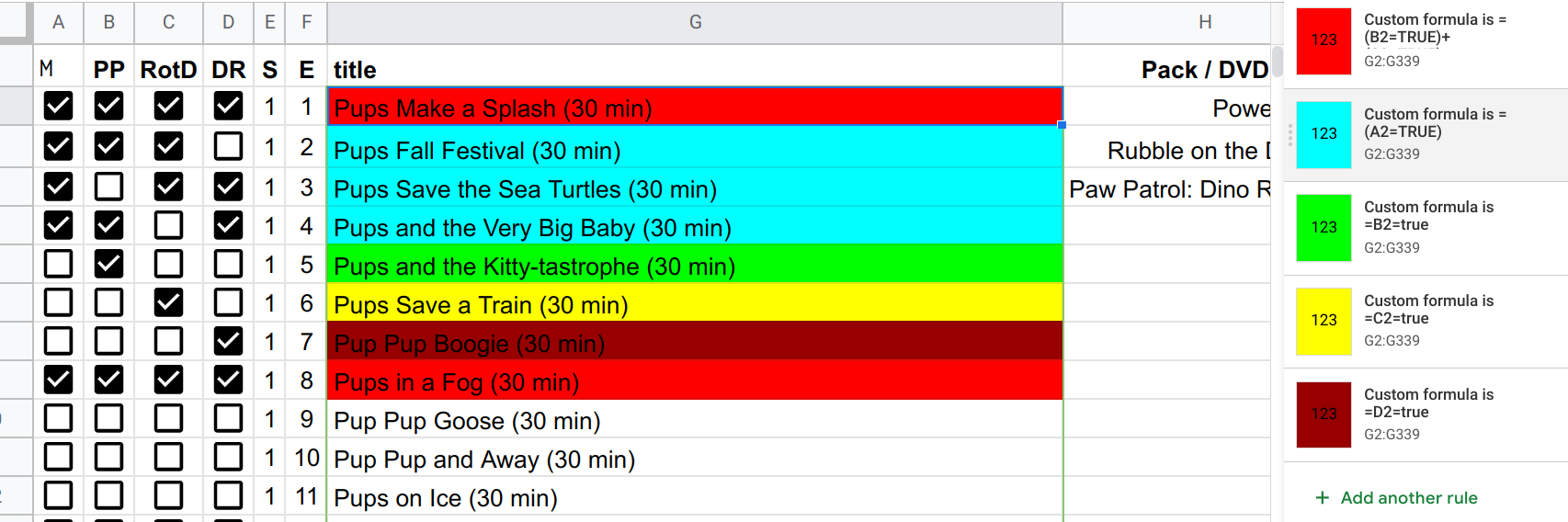

If this is correct, try the following.
The order of your rules is very important. We want to check for all three checked first, then for any two, and lastly, for each individual checkbox, in columns B-D.
So the first rule, for red, should be a custom formula like this:
=(B2=TRUE)+(C2=TRUE)+(D2=TRUE)>2For two boxes checked, we now just need to see if column A is "checked". Yes, it will also have been checked if all three columns were checked, but we covered that with the first rule. If that rule wasn't triggered, then we now now that it means only two (or fewer) are checked. I've used baby blue for this condition.
=(A2=TRUE)And lastly you already had three rules working for the individual columns.
Remember, the rules have to be in this order. To move a rule up or down, hover over the left edge of the rule, (when looking at the list of rules) and then click and hold, to be able to slide it up or down, above or below another rule in the list.
Let me know if this helps. If you have any issues, post back and please change your sheet options so that anyone can EDIT.
Cheers,
Gill
When you've received a response that answers your question, please observe these forum courtesies;
• Leave your demo sheet shared as part of this solution's archive,
• Click Recommend on the post that best addressed your question, and
• Post again soon!
Original Poster Owen R marked this as an answer
Helpful?Upvote Downvote
All Replies (5)
Hi Owen,
This may help. Your sheet is view only, so I can't help directly, but go to cell A1, and delete everything in A1 to the bottom of the column. If unsure how, while in A1, select <Ctrl>-Shift and then <Down-arrow> several times until you are at the bottom of column A. Then press Delete.
Next, paste the following formula in A1.
={"M";ArrayFormula( IF((--B2:B)*(--C2:C) +(--B2:B)*(--D2:D) +(--C2:C)*(--D2:D)>0,TRUE,FALSE))}Then go back and select column A from A2 down to the bottom. Then Insert - Checkbox from the menu.
This should now turn "on" when two or more of the checkboxes in columns B-D are checked, in a given row.
And for your conditional formatting, see the following image.
If this is correct, try the following.
The order of your rules is very important. We want to check for all three checked first, then for any two, and lastly, for each individual checkbox, in columns B-D.
So the first rule, for red, should be a custom formula like this:
=(B2=TRUE)+(C2=TRUE)+(D2=TRUE)>2For two boxes checked, we now just need to see if column A is "checked". Yes, it will also have been checked if all three columns were checked, but we covered that with the first rule. If that rule wasn't triggered, then we now now that it means only two (or fewer) are checked. I've used baby blue for this condition.
=(A2=TRUE)And lastly you already had three rules working for the individual columns.
Remember, the rules have to be in this order. To move a rule up or down, hover over the left edge of the rule, (when looking at the list of rules) and then click and hold, to be able to slide it up or down, above or below another rule in the list.
Let me know if this helps. If you have any issues, post back and please change your sheet options so that anyone can EDIT.
Cheers,
Gill
When you've received a response that answers your question, please observe these forum courtesies;
• Leave your demo sheet shared as part of this solution's archive,
• Click Recommend on the post that best addressed your question, and
• Post again soon!
Original Poster Owen R marked this as an answer
Mar 10, 2021
Additionally I found one other issue with the way I was doing things, for the Unique Episodes I was simply adding up the column for how many episodes are checked, and then subtracting the total from Column A. However I just realized that is giving inaccurate information, since column D has 6 check boxes, and column A also has 6 but there are 3 unique boxes ticked for column D. What I need to be able to do is ascertain if there are 6 boxes ticked in column D, to check and see if any of THOSE boxes correspond to columns B or C.
I have updated the sheet to show an example. Rows 2 and 3 should NOT be counted because there are corresponding checks in either column B or C. However the Unique Episodes should show 1 because there is only column D selected on Row 4. (outside of this example it should show 5 total right now because there are 5 unique episodes from the rest of the list.
The sheet should be editable now.
Hi Owen,
First, to count the unique ones (I think that means those where ONLY column D is checked), try this formula, which I've put in K2:
=QUERY(A2:D, "select count(D) where D=TRUE and B=FALSE and C=FALSE label count(D) '' ",0)It's probably pretty clear what it does, so should be easy to modify, but let me know if you have any questions.
See also the tab I added, and where I applied a data filter, just to make it easy to see only the rows with checkboxes marked. Currently, I'm showing all rows with column D checked.
Then, to explain the formula in A1:
={"M"; ArrayFormula( IF( (--B2:B)*(--C2:C) + (--B2:B)*(--D2:D) + (--C2:C)*(--D2:D) >0, TRUE,FALSE))}To be able to put the formula up in the "header" row, instead of in the first data row, which is typically done, I needed to included the header label, ie. "M"
So I start by building a virtual array, {....}, which is going to fill multiple cells, in this case the whole of column A.
So the first element in the virtual array is the header, "M", followed by a semi-colon to jump down to the next row. (To learn more about virtual array's, read this post by our expert Lance)
Then I want to find out if two (or more) of columns B, C, and D are checked.
=IF(B2, "if true...", "if false...") is the simplest form. If B2 equates to TRUE, do something. B2 will equate to TRUE if it has any number greater than zero, or is equal to TRUE for some other reason. In our case, it will be TRUE if it is checked.
But we want to turn the TRUE value into a "1", so we can add them up to see whether we have more than one checked. Putting a double negative in front of a TRUE or FALSE value is a method of converting it to zero or one.
Then, 1 times 1 = 1, but 1 * 0 = 0. So if I do (B2 * C2), if they are both equal to 1 we get 1, but if either one of them is zero we get zero. So we do that for all three possibilities, B and C, B and D, and C and D. As long as the sum of those is 1 or more, than it means that at least two of them were checked. Otherwise, if only zero or one were checked, we'd have 0 + 0 + 0.
I hope you followed that! Then, assuming at least two were checked, we set that cell (in column A) equal to TRUE.
And lastly, we do all of this under an array formula, which applies it all the way down the range. That's why all of our cell references are in the form of B2:B.
I hope this has helped. Let me know if still unclear. ARRAYFORMULAs are used extensively to simplify filling columns with data, as well as for cycling through data to generate unique results.
Cheers,
Gill
Original Poster Owen R marked this as an answer
Mar 10, 2021
Also thank you for the explanation of the column A, that should help with adding additional columns as well.
Mar 10, 2021
Owen,
I'm glad I could help, and thanks for the feedback and recommendation. Much appreciated by us volunteer contributors here on the forum!
Good luck, and post back anytime with new questions.
Cheers,
Gill